3. The Network Model

This chapter discusses how EPANET models the physical objects that constitute a distribution system as well as its operational parameters. Details about how this information is entered into the program are presented in later chapters. An overview is also given on the computational methods that EPANET uses to simulate hydraulic and water quality transport behavior.

---

3.1. Physical Components

EPANET models a water distribution system as a collection of links connected to nodes. The links represent pipes, pumps, and control valves. The nodes represent junctions, tanks, and reservoirs. Fig. 3.1 below illustrates how these objects can be connected to one another to form a network.

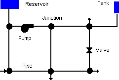
Fig. 3.1 Physical Components in a Water Distribution System.

Junctions

Junctions are points in the network where links join together and where water enters or leaves the network. The basic input data required for junctions are:

• Elevation above some reference (usually mean sea level)
• Water demand (rate of withdrawal from the network)
• Initial water quality

The output results computed for junctions at all time periods of a simulation are:

• Hydraulic head (internal energy per unit weight of fluid)
• Pressure
• Water quality

Junctions can also:

• Have their demand vary with time
• Have multiple categories of demands assigned to them
• Have negative demands indicating that water is entering the network
• Have pressure driven demand
• Be water quality sources where constituents enter the network
• Contain emitters (or sprinklers) which make the outflow rate depend on the pressure

Reservoirs

Reservoirs are nodes that represent an infinite external source or sink of water to the network. They are used to model such things as lakes, rivers, groundwater aquifers, and tie-ins to other systems. Reservoirs can also serve as water quality source points.

The primary input properties for a reservoir are its hydraulic head (equal to the water surface elevation if the reservoir is not under pressure) and its initial quality for water quality analysis.

Because a reservoir is a boundary point to a network, its head and water quality cannot be affected by what happens within the network. Therefore it has no computed output properties. However its head can be made to vary with time by assigning a time pattern to it (see Time Patterns below).

Tanks

Tanks are nodes with storage capacity, where the volume of stored water can vary with time during a simulation. The primary input properties for tanks are:

• Bottom elevation (where water level is zero)
• Diameter (or shape if non-cylindrical )
• Initial, minimum and maximum water levels
• Initial water quality

The principal outputs computed over time are:

• Hydraulic head (water surface elevation)
• Water quality

Tanks are required to operate within their minimum and maximum levels. EPANET stops outflow if a tank is at its minimum level and stops inflow if it is at its maximum level. Tanks can also serve as water quality source points.

Emitters

Emitters are devices associated with junctions that model the flow through a nozzle or orifice that discharges to the atmosphere. The flow rate through the emitter varies as a function of the pressure available at the node:

\[q = C p^{\gamma}\]

where \(q\) = flow rate, \(p\) = pressure, \(C\) = discharge coefficient, and \(\gamma\) = pressure exponent. For nozzles and sprinkler heads \(\gamma\) equals 0.5 and the manufacturer usually provides the value of the discharge coefficient in units of gpm/psi ^0.5 (stated as the flow through the device at a 1 psi pressure drop).

Emitters are used to model flow through sprinkler systems and irrigation networks. They can also be used to simulate leakage in a pipe connected to the junction (if a discharge coefficient and pressure exponent for the leaking crack or joint can be estimated) or compute a fire flow at the junction (the flow available at some minimum residual pressure). In the latter case one would use a very high value of the discharge coefficient (e.g., 100 times the maximum flow expected) and modify the junction’s elevation to include the equivalent head of the pressure target. EPANET treats emitters as a property of a junction and not as a separate network component.

Note

The pressure-flow relation at a junction defined by an emitter should not be confused with the pressure-demand relation when performing a pressure driven analysis (PDA). See Hydraulic Simulation Model for more information.

Pipes

Pipes are links that convey water from one point in the network to another. EPANET assumes that all pipes are full at all times. Flow direction is from the end at higher hydraulic head (internal energy per weight of water) to that at lower head. The principal hydraulic input parameters for pipes are:

• Start and end nodes
• Diameter
• Length
• Roughness coefficient (for determining headloss)
• Status (open, closed, or contains a check valve)

The status parameter allows pipes to implicitly contain shutoff (gate) valves and check (non-return) valves (which allow flow in only one direction).

The water quality inputs for pipes consist of:

• Bulk reaction coefficient
• Wall reaction coefficient

These coefficients are explained more thoroughly in Section 3.4 below.

Computed outputs for pipes include:

• Flow rate
• Velocity
• Headloss
• Darcy-Weisbach friction factor
• Average reaction rate (over the pipe length)
• Average water quality (over the pipe length)

The hydraulic head lost by water flowing in a pipe due to friction with the pipe walls can be computed using one of three different formulas:

• Hazen-Williams formula
• Darcy-Weisbach formula
• Chezy-Manning formula

The Hazen-Williams formula is the most commonly used headloss formula in the US. It cannot be used for liquids other than water and was originally developed for turbulent flow only. The Darcy-Weisbach formula is the most theoretically correct. It applies over all flow regimes and to all liquids. The Chezy-Manning formula is more commonly used for open channel flow.

Each formula uses the following equation to compute headloss between the start and end node of the pipe:

\[h_{L} = A q^{B}\]

where \(h_{L}\) = headloss (Length), \(q\) = flow rate (Volume/Time), \(A\) = resistance coefficient, and \(B\) = flow exponent. Table 3.1 lists expressions for the resistance coefficient and values for the flow exponent for each of the formulas. Each formula uses a different pipe roughness coefficient that must be determined empirically. Table 3.2 lists general ranges of these coefficients for different types of new pipe materials. Be aware that a pipe’s roughness coefficient can change considerably with age.

With the Darcy-Weisbach formula EPANET uses different methods to compute the friction factor f depending on the flow regime:

• The Hagen–Poiseuille formula is used for laminar flow (Re < 2,000).
• The Swamee and Jain approximation to the Colebrook-White equation is used for fully turbulent flow (Re > 4,000).
• A cubic interpolation from the Moody Diagram is used for transitional flow (2,000 < Re < 4,000).

Consult Chapter Analysis Algorithms for the actual equations used.

Table 3.1 Pipe Headloss Formulas for Full Flow (for headloss in feet and flow rate in cfs)

Formula	Resistance Coefficient (\(A\))	Flow Exponent (\(B\))
Hazen-Williams	\(4.727\,C^{-1.852}\,d^{-4.871}\,L\)	\(1.852\)
Darcy-Weisbach	\(0.0252\,f(\epsilon,d,q)\,d ^{-5}\,L\)	\(2\)
Chezy-Manning	\(4.66\,n^{2}\,d^{-5.33}\,L\)	\(2\)

Notes:

\(C\) = Hazen-Williams roughness coefficient

\(\epsilon\) = Darcy-Weisbach roughness coefficient (ft)

\(f\) = friction factor (dependent on \(\epsilon\), \(d\), and \(q\))

\(n\) = Manning roughness coefficient

\(d\) = pipe diameter (ft)

\(L\) = pipe length (ft)

\(q\) = flow rate (cfs)

Table 3.2 Roughness Coefficients for New Pipe

Material	Hazen-Williams \(C\) (unitless)	Darcy-Weisbach \(\epsilon\) (ft x \(10^{-3}\))	Manning’s \(n\) (unitless)
Cast Iron	130 – 140	0.85	0.012 – 0.015
Concrete or Concrete Lined	120 – 140	1.0 – 10	0.012 – 0.017
Galvanized Iron	120	0.5	0.015 – 0.017
Plastic	140 – 150	0.005	0.011 – 0.015
Steel	140 – 150	0.15	0.015 – 0.017
Vitrified Clay	110		0.013 – 0.015

Pipes can be set open or closed at preset times or when specific conditions exist, such as when tank levels fall below or above certain set points, or when nodal pressures fall below or above certain values. See the discussion of Controls in Section 3.2.

Minor Losses

Minor head losses (also called local losses) are caused by the added turbulence that occurs at bends and fittings. The importance of including such losses depends on the layout of the network and the degree of accuracy required. They can be accounted for by assigning the pipe a minor loss coefficient. The minor headloss becomes the product of this coefficient and the velocity head of the pipe, i.e.,

\[h_L = K (\frac{v^2}{2g})\]

where \(K\) = minor loss coefficient, \(v\) = flow velocity (Length/Time), and \(g\) = acceleration of gravity (Length/Time ²). Table 3.3 provides minor loss coefficients for several types of fittings.

Table 3.3 Minor Loss Coefficients for Selected Fittings

FITTING	LOSS COEFFICIENT
Globe valve, fully open	10.0
Angle valve, fully open	5.0
Swing check valve, fully open	2.5
Gate valve, fully open	0.2
Short-radius elbow	0.9
Medium-radius elbow	0.8
Long-radius elbow	0.6
45 degree elbow	0.4
Closed return bend	2.2
Standard tee - flow through run	0.6
Standard tee - flow through branch	1.8
Square entrance	0.5
Exit	1.0

Pumps

Pumps are links that impart energy to a fluid thereby raising its hydraulic head. The principal input parameters for a pump are its start and end nodes and its pump curve (the combination of heads and flows that the pump can produce). In lieu of a pump curve, the pump could be represented as a constant energy device, one that supplies a constant amount of energy (horsepower or kilowatts) to the fluid for all combinations of flow and head.

The principal output parameters are flow and head gain. Flow through a pump is unidirectional and EPANET will not allow a pump to operate outside the range of its pump curve.

Variable speed pumps can also be considered by specifying that their speed setting be changed under these same types of conditions. By definition, the original pump curve supplied to the program has a relative speed setting of 1. If the pump speed doubles, then the relative setting would be 2; if run at half speed, the relative setting is 0.5 and so on. Changing the pump speed shifts the position and shape of the pump curve (see the section on Pump Curves below).

As with pipes, pumps can be turned on and off at preset times or when certain conditions exist in the network. A pump’s operation can also be described by assigning it a time pattern of relative speed settings. EPANET can also compute the energy consumption and cost of a pump. Each pump can be assigned an efficiency curve and schedule of energy prices. If these are not supplied then a set of global energy options will be used.

Flow through a pump is unidirectional. If system conditions require more head than the pump can produce, EPANET shuts the pump off. If more than the maximum flow is required, EPANET extrapolates the pump curve to the required flow, even if this produces a negative head. In both cases a warning message will be issued.

Valves

Valves are links that limit the pressure or flow at a specific point in the network. Their principal input parameters include:

• Start and end nodes
• Diameter
• Setting
• Status

The computed outputs for a valve are flow rate and headloss. The different types of valves included in EPANET are:

• Pressure Reducing Valve (PRV)
• Pressure Sustaining Valve (PSV)
• Pressure Breaker Valve (PBV)
• Flow Control Valve (FCV)
• Throttle Control Valve (TCV)
• General Purpose Valve (GPV)

PRVs limit the pressure at a point in the pipe network. EPANET computes in which of three different states a PRV can be in:

• Partially opened (i.e., active) to achieve its pressure setting on its downstream side when the upstream pressure is above the setting
• Fully open if the upstream pressure is below the setting
• Closed if the pressure on the downstream side exceeds that on the upstream side (i.e., reverse flow is not allowed)

PSVs maintain a set pressure at a specific point in the pipe network. EPANET computes in which of three different states a PSV can be in:

• Partially opened (i.e., active) to maintain its pressure setting on its upstream side when the downstream pressure is below this value
• Fully open if the downstream pressure is above the setting
• Closed if the pressure on the downstream side exceeds that on the upstream side (i.e., reverse flow is not allowed)

PBVs force a specified pressure loss to occur across the valve. Flow through the valve can be in either direction. PBV’s are not true physical devices but can be used to model situations where a particular pressure drop is known to exist.

FCVs limit the flow to a specified amount. The program produces a warning message if this flow cannot be maintained without having to add additional head at the valve (i.e., the flow cannot be maintained even with the valve fully open).

TCVs simulate a partially closed valve by adjusting the minor head loss coefficient of the valve. A relationship between the degree to which a valve is closed and the resulting head loss coefficient is usually available from the valve manufacturer.

GPVs are used to represent a link where the user supplies a special flow - head loss relationship instead of following one of the standard hydraulic formulas. They can be used to model turbines, well draw-down or reduced-flow backflow prevention valves.

Shutoff (gate) valves and check (non-return) valves, which completely open or close pipes, are not considered as separate valve links but are instead included as a property of the pipe in which they are placed.

Each type of valve has a different type of setting parameter that describes its operating point (pressure for PRVs, PSVs, and PBVs; flow for FCVs; loss coefficient for TCVs, and head loss curve for GPVs).

Valves can have their control status overridden by specifying they be either completely open or completely closed. A valve’s status and its setting can be changed during the simulation by using control statements.

Because of the ways in which valves are modeled the following rules apply when adding valves to a network:

• A PRV, PSV or FCV cannot be directly connected to a reservoir or tank (use a length of pipe to separate the two)
• PRVs cannot share the same downstream node or be linked in series
• Two PSVs cannot share the same upstream node or be linked in series
• A PSV cannot be connected to the downstream node of a PRV

3.2. Non-Physical Components

In addition to physical components, EPANET employs three types of informational objects – curves, patterns, and controls - that describe the behavior and operational aspects of a distribution system.

Curves

Curves are objects that contain data pairs representing a relationship between two quantities. Two or more objects can share the same curve. An EPANET model can utilize the following types of curves:

• Pump Curve
• Efficiency Curve
• Volume Curve
• Head Loss Curve Pump Curve

Pump Curve

A Pump Curve represents the relationship between the head and flow rate that a pump can deliver at its nominal speed setting. Head is the head gain imparted to the water by the pump and is plotted on the vertical (Y) axis of the curve in feet (meters). Flow rate is plotted on the horizontal (X) axis in flow units. A valid pump curve must have decreasing head with increasing flow.

EPANET will use a different shape of pump curve depending on the number of points supplied.

Single-Point Curve – A single-point pump curve is defined by a single head-flow combination that represents a pump’s desired operating point. EPANET adds two more points to the curve by assuming a shutoff head at zero flow equal to 133% of the design head and a maximum flow at zero head equal to twice the design flow. It then treats the curve as a three-point curve. Fig. 3.2 shows an example of a single-point pump curve.

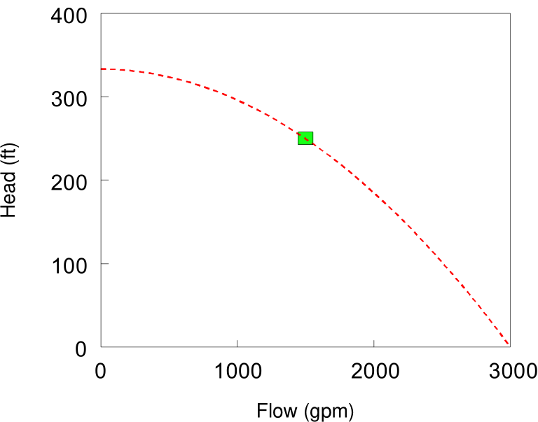
Fig. 3.2 Single-point Pump Curve.

Three-Point Curve – A three-point pump curve is defined by three operating points: a Low Flow point (flow and head at low or zero flow condition), a Design Flow point (flow and head at desired operating point), and a Maximum Flow point (flow and head at maximum flow). EPANET tries to fit a continuous function of the form

\[h_{G} = A - B \, q^{C}\]

through the three points to define the entire pump curve. In this function, \(h_{g}\) = head gain, \(q\) = flow rate, and \(A\), \(B\), and \(C\) are constants. Fig. 3.3 shows an example of a three-point pump curve.

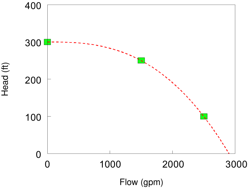
Fig. 3.3 Three-point Pump Curve.

Multi-Point Curve – A multi-point pump curve is defined by providing either a pair of head-flow points or four or more such points. EPANET creates a complete curve by connecting the points with straight-line segments. Fig. 3.4 shows an example of a multi-point pump curve.

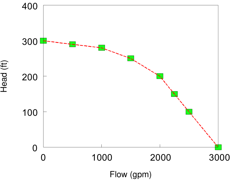
Fig. 3.4 Multi-point Pump Curve.

For variable speed pumps, the pump curve shifts as the speed changes. The relationships between flow (\(Q\)) and head (\(H\)) at speeds \(N1\) and \(N2\) are

\[\begin{split}\begin{gathered} \frac{Q_1}{Q_2} = \frac{N_1}{N_2} \\ \frac{H_1}{H_2} = \left( \frac{N_1}{N_2} \right)^2 \end{gathered}\end{split}\]

Fig. 3.5 shows an example of a variable-speed pump curve.

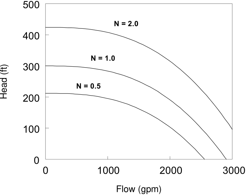
Fig. 3.5 Variable-speed Pump Curve.

Efficiency Curve

An Efficiency Curve determines pump efficiency (Y in percent) as a function of pump flow rate (X in flow units). An example efficiency curve is shown in Fig. 3.6. Efficiency should represent wire-to-water efficiency that takes into account mechanical losses in the pump itself as well as electrical losses in the pump’s motor. The curve is used only for energy calculations. If not supplied for a specific pump then a fixed global pump efficiency will be used.

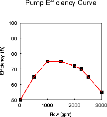
Fig. 3.6 Pump Efficiency Curve.

Volume Curve

A Volume Curve determines how storage tank volume (Y in cubic feet or cubic meters) varies as a function of water level (X in feet or meters). It is used when it is necessary to accurately represent tanks whose cross-sectional area varies with height. The lower and upper water levels supplied for the curve must contain the lower and upper levels between which the tank operates. An example of a tank volume curve is given in Fig. 3.7.

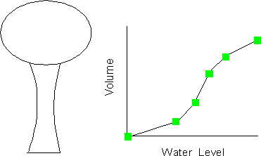
Fig. 3.7 Tank Volume Curve.

Headloss Curve

A Headloss Curve is used to described the headloss (Y in feet or meters) through a General Purpose Valve (GPV) as a function of flow rate (X in flow units). It provides the capability to model devices and situations with unique headloss-flow relationships, such as reduced flow - backflow prevention valves, turbines, and well draw-down behavior.

Time Patterns

A Time Pattern is a collection of multipliers that can be applied to a quantity to allow it to vary over time. Nodal demands, reservoir heads, pump schedules, and water quality source inputs can all have time patterns associated with them. The time interval used in all patterns is a fixed value, set with the project’s Time Options (see Section 8.1). Within this interval a quantity remains at a constant level, equal to the product of its nominal value and the pattern’s multiplier for that time period. Although all time patterns must utilize the same time interval, each can have a different number of periods. When the simulation clock exceeds the number of periods in a pattern, the pattern wraps around to its first period again.

As an example of how time patterns work consider a junction node with an average demand of 10 GPM. Assume that the time pattern interval has been set to 4 hours and a pattern with the following multipliers has been specified for demand at this node:

Period	1	2	3	4	5	6
Multiplier	0.5	0.8	1.0	1.2	0.9	0.7

Then during the simulation the actual demand exerted at this node will be as follows:

Hours	0-4	4-8	8-12	12-16	16-20	20-24	24-28
Demand	5	8	10	12	9	7	5

Controls

Controls are statements that determine how the network is operated over time. They specify the status of selected links as a function of time, tank water levels, and pressures at select points within the network. There are two categories of controls that can be used:

• Simple Controls
• Rule-Based Controls Simple Controls

Simple Controls

Simple controls change the status or setting of a link based on:

• The water level in a tank

• The pressure at a junction
• The time into the simulation
• The time of day

They are statements expressed in one of the following three formats:

LINK x status IF NODE y ABOVE/BELOW z
LINK x status AT TIME t
LINK x status AT CLOCKTIME c AM/PM

where:

x = a link ID label,

status = OPEN or CLOSED, a pump speed setting, or a control valve setting,

y = a node ID label,

z = a pressure for a junction or a water level for a tank,

t = a time since the start of the simulation (decimal hours or hours:minutes),

c = a 24-hour clock time.

Some examples of simple controls are (Table 3.4):

Table 3.4 Examples of Simple Controls

Control Statement	Meaning
LINK 12 CLOSED IF NODE 23 ABOVE 20	(Close Link 12 when the level in Tank 23 exceeds 20 ft.)
LINK 12 OPEN IF NODE 130 BELOW 30	(Open Link 12 if the pressure at Node 130 drops below 30 psi)
LINK 12 1.5 AT TIME 16	(Set the relative speed of pump 12 to 1.5 at 16 hours into the simulation)
LINK 12 CLOSED AT CLOCKTIME 10 AM LINK 12 OPEN AT CLOCKTIME 8 PM	(Link 12 is repeatedly closed at 10 AM and opened at 8 PM throughout the simulation)

There is no limit on the number of simple control statements that can be used.

Note: Level controls are stated in terms of the height of water above the tank bottom, not the elevation (total head) of the water surface.

Note: Using a pair of pressure controls to open and close a link can cause the system to become unstable if the pressure settings are too close to one another. In this case using a pair of Rule-Based controls might provide more stability.

Rule-Based Controls

Rule-Based Controls allow link status and settings to be based on a combination of conditions that might exist in the network after an initial hydraulic state of the system is computed. Here are several examples of Rule-Based Controls:

Example 1:

This set of rules shuts down a pump and opens a by-pass pipe when the level in a tank exceeds a certain value and does the opposite when the level is below another value.

RULE 1
IF TANK 1 LEVEL ABOVE 19.1
THEN PUMP 335 STATUS IS CLOSED
AND PIPE 330 STATUS IS OPEN

RULE 2
IF TANK 1 LEVEL BELOW 17.1
THEN PUMP 335 STATUS IS OPEN
AND PIPE 330 STATUS IS CLOSED

Example 2:

These rules change the tank level at which a pump turns on depending on the time of day.

RULE 3
IF SYSTEM CLOCKTIME >= 8 AM
AND SYSTEM CLOCKTIME < 6 PM
AND TANK 1 LEVEL BELOW 12
THEN PUMP 335 STATUS IS OPEN

RULE 4
IF SYSTEM CLOCKTIME >= 6 PM
OR SYSTEM CLOCKTIME < 8 AM
AND TANK 1 LEVEL BELOW 14
THEN PUMP 335 STATUS IS OPEN

A description of the formats used with Rule-Based controls can be found in Appendix Command Line EPANET, under the [RULES] heading.

3.3. Hydraulic Simulation Model

EPANET’s hydraulic simulation model computes hydraulic heads at junctions and flow rates through links for a fixed set of reservoir levels, tank levels, and water demands over a succession of points in time. From one time step to the next reservoir levels and junction demands are updated according to their prescribed time patterns while tank levels are updated using the current flow solution. The solution for heads and flows at a particular point in time involves solving simultaneously the conservation of flow equation for each junction and the head loss relationship across each link in the network. This process, known as hydraulically balancing the network, requires using an iterative technique to solve the nonlinear equations involved. EPANET employs the Global Gradient Algorithm for this purpose. EPANET employs the “Gradient Algorithm” for this purpose. Consult Chapter Analysis Algorithms for details.

The hydraulic time step used for extended period simulation (EPS) can be set by the user. A typical value is 1 hour. Shorter time steps than normal will occur automatically whenever one of the following events occurs:

• The next output reporting time period occurs
• The next time pattern period occurs
• A tank becomes empty or full
• A simple control or rule-based control is activated

EPANET’s hydraulic analysis allows for two different ways of modeling water demands (i.e., consumption) at network junction nodes. Demand Driven Analysis (DDA) requires that demands at each point in time are fixed values that must be delivered no matter what nodal pressures and link flows are produced by a hydraulic solution. This has been the classical approach used to model demands, but it can result in situations where required demands are satisfied at nodes with negative pressures - a physical impossibility. An alternative approach, known as Pressure Driven Analysis (PDA), allows the actual demand delivered at a node to depend on the node’s pressure. Below some minimum pressure demand is zero, above some service pressure the full required demand is supplied and in between demand varies as a power law function of pressure. Using PDA is one way to avoid having positive demands at nodes with negative pressures.

EPANET’s Hydraulic Analysis Options are used to select a choice of demand model and to supply the parameters used by PDA.

3.4. Water Quality Simulation Model

Basic Transport

EPANET’s water quality simulator uses a Lagrangian time-based approach to track the fate of discrete parcels of water as they move along pipes and mix together at junctions between fixed-length time steps. These water quality time steps are typically much shorter than the hydraulic time step (e.g., minutes rather than hours) to accommodate the short times of travel that can occur within pipes.

The method tracks the concentration and size of a series of non-overlapping segments of water that fills each link of the network. As time progresses, the size of the most upstream segment in a link increases as water enters the link while an equal loss in size of the most downstream segment occurs as water leaves the link. The size of the segments in between these remains unchanged.

For each water quality time step, the contents of each segment are subjected to reaction, a cumulative account is kept of the total mass and flow volume entering each node, and the positions of the segments are updated. New node concentrations are then calculated, which include the contributions from any external sources. Storage tank concentrations are updated depending on the type of mixing model that is used (see below). Finally, a new segment will be created at the end of each link that receives inflow from a node if the new node quality differs by a user-specified tolerance from that of the link’s last segment.

Initially each pipe in the network consists of a single segment whose quality equals the initial quality assigned to the upstream node. Whenever there is a flow reversal in a pipe, the pipe’s parcels are re-ordered from front to back.

Water Quality Sources

Water quality sources are nodes where the quality of external flow entering the network is specified. They can represent the main treatment works, a well-head or satellite treatment facility, or an unwanted contaminant intrusion. Source quality can be made to vary over time by assigning it a time pattern. EPANET can model the following types of sources:

• A concentration source fixes the concentration of any external inflow entering the network at a node, such as flow from a reservoir or from a negative demand placed at a junction.
• A mass booster source adds a fixed mass flow to that entering the node from other points in the network.
• A set point booster source fixes the concentration of any flow leaving the node (as long as the concentration resulting from all inflow to the node is below the setpoint).
• A flow paced booster source adds a fixed concentration to that resulting from the mixing of all inflow to the node from other points in the network

The concentration-type source is best used for nodes that represent source water supplies or treatment works (e.g., reservoirs or nodes assigned a negative demand). The booster-type source is best used to model direct injection of a tracer or additional disinfectant into the network or to model a contaminant intrusion.

Mixing in Storage Tanks

EPANET can use four different types of models to characterize mixing within storage tanks:

• Complete Mixing
• Two-Compartment Mixing
• First-in First-out (FIFO) Plug Flow
• Last-in First-out (LIFO) Plug Flow

Different models can be used with different tanks within a network.

The Complete Mixing model (Fig. 3.8) assumes that all water that enters a tank is instantaneously and completely mixed with the water already in the tank. It is the simplest form of mixing behavior to assume, requires no extra parameters to describe it, and seems to apply quite well to a large number of facilities that operate in fill-and-draw fashion.

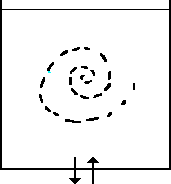
Fig. 3.8 Complete Mixing.

The Two-Compartment Mixing model (Fig. 3.9) divides the available storage volume in a tank into two compartments, both of which are assumed completely mixed. The inlet/outlet pipes of the tank are assumed to be located in the first compartment. New water that enters the tank mixes with the water in the first compartment. If this compartment is full, then it sends its overflow to the second compartment where it completely mixes with the water already stored there. When water leaves the tank, it exits from the first compartment, which if full, receives an equivalent amount of water from the second compartment to make up the difference. The first compartment is capable of simulating short-circuiting between inflow and outflow while the second compartment can represent dead zones. The user must supply a single parameter, which is the fraction of the total tank volume devoted to the first compartment.

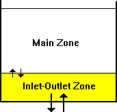
Fig. 3.9 Two-compartment Mixing.

The FIFO Plug Flow model (Fig. 3.10) assumes that there is no mixing of water at all during its residence time in a tank. Water parcels move through the tank in a segregated fashion where the first parcel to enter is also the first to leave. Physically speaking, this model is most appropriate for baffled tanks that operate with simultaneous inflow and outflow. There are no additional parameters needed to describe this mixing model.

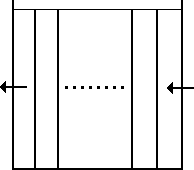
Fig. 3.10 Plug Flow - FIFO.

The LIFO Plug Flow model (Fig. 3.11) also assumes that there is no mixing between parcels of water that enter a tank. However in contrast to FIFO Plug Flow, the water parcels stack up one on top of another, where water enters and leaves the tank on the bottom. This type of model might apply to a tall, narrow standpipe with an inlet/outlet pipe at the bottom and a low momentum inflow. It requires no additional parameters be provided.

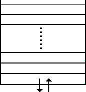
Fig. 3.11 Plug Flow - LIFO.

Water Quality Reactions

EPANET can track the growth or decay of a substance by reaction as it travels through a distribution system. In order to do this it needs to know the rate at which the substance reacts and how this rate might depend on substance concentration. Reactions can occur both within the bulk flow and with material along the pipe wall. This is illustrated in Fig. 3.12. In this example free chlorine (HOCl) is shown reacting with natural organic matter (NOM) in the bulk phase and is also transported through a boundary layer at the pipe wall to oxidize iron (Fe) released from pipe wall corrosion. Bulk fluid reactions can also occur within tanks. EPANET allows a modeler to treat these two reaction zones separately.

Fig. 3.12 Reaction zones within a pipe.

Bulk Reactions

EPANET models reactions occurring in the bulk flow with n-th order kinetics, where the instantaneous rate of reaction (\(R\) in mass/volume/time) is assumed to be concentration-dependent according to

\[R = K_{b} C^{n}\]

Here \(K_{b}\) = a bulk reaction rate coefficient, \(C\) = reactant concentration (mass/volume), and \(n\) = a reaction order. \(K_b\) has units of concentration raised to the \((1 - n)\) power divided by time. It is positive for growth reactions and negative for decay reactions.

EPANET can also consider reactions where a limiting concentration exists on the ultimate growth or loss of the substance. In this case the rate expression becomes

\[\begin{gathered} R = K_{b} (C_{L} - C) \times C^{(n - 1)} : n > 0, K_{b} > 0 \end{gathered}\]

\[\begin{gathered} R = K_{b} (C - C_{L} ) \times C^{(n - 1)} : n > 0, K_{b} < 0 \end{gathered}\]

where \(C_L\) = the limiting concentration. Thus there are three parameters (\(K_b\), \(C_L\), and \(n\)) that are used to characterize bulk reaction rates. Some special cases of well-known kinetic models are provided in Table 3.5 (see Section 12.2 for more examples):

Table 3.5 Special Cases of Well-known Kinetic Models

Model	Parameters	Examples
First-Order Decay	\(C_L = 0, K_b < 0, n = 1\)	Chlorine
First-Order Saturation Growth	\(C_L > 0, K_b > 0, n = 1\)	Trihalomethanes
Zero-Order Kinetics	\(C_L = 0, K_b <> 0, n = 0\)	Water Age
No Reaction	\(C_L = 0, K_b = 0\)	Fluoride Tracer

The \(K_b\) for first-order reactions can be estimated by placing a sample of water in a series of non-reacting glass bottles and analyzing the contents of each bottle at different points in time. If the reaction is first-order, then plotting the natural log \((C_t / C_0)\) against time should result in a straight line, where \(C_t\) is concentration at time \(t\) and \(C_0\) is concentration at time zero. \(K_b\) would then be estimated as the slope of this line.

Bulk reaction coefficients usually increase with increasing temperature. Running multiple bottle tests at different temperatures will provide more accurate assessment of how the rate coefficient varies with temperature

Wall Reactions

The rate of water quality reactions occurring at or near the pipe wall can be considered to be dependent on the concentration in the bulk flow by using an expression of the form

\[R = ( A / V ) K_{w} C^{n}\]

where \(K_{w}\) = a wall reaction rate coefficient and \((A / V)\) = the surface area per unit volume within a pipe (equal to 4 divided by the pipe diameter). The latter term converts the mass reacting per unit of wall area to a per unit volume basis. EPANET limits the choice of wall reaction order to either 0 or 1, so that the units of \(K_{w}\) are either mass/area/time or length/time, respectively. As with \(K_{b}\), \(K_{w}\) must be supplied to the program by the modeler. First-order \(K_{w}\) values can range anywhere from 0 to as much as 5 ft/day.

The variable \(K_{w}\) should be adjusted to account for any mass transfer limitations in moving reactants and products between the bulk flow and the wall. EPANET does this automatically, basing the adjustment on the molecular diffusivity of the substance being modeled and on the flow’s Reynolds number. See Section 12.2 for details. (Setting the molecular diffusivity to zero will cause mass transfer effects to be ignored.)

The wall reaction coefficient can depend on temperature and can also be correlated to pipe age and material. It is well known that as metal pipes age their roughness tends to increase due to encrustation and tuburculation of corrosion products on the pipe walls. This increase in roughness produces a lower Hazen-Williams C-factor or a higher Darcy-Weisbach roughness coefficient, resulting in greater frictional head loss in flow through the pipe.

There is some evidence to suggest that the same processes that increase a pipe’s roughness with age also tend to increase the reactivity of its wall with some chemical species, particularly chlorine and other disinfectants. EPANET can make each pipe’s \(K_{w}\) be a function of the coefficient used to describe its roughness. A different function applies depending on the formula used to compute headloss through the pipe (Table 3.6):

Table 3.6 Wall Reaction Formulas Related to Headloss Formula

Headloss Formula	Wall Reaction Formula
Hazen-Williams	\(K_w = F / C\)
Darcy-Weisbach	\(K_w = -F / \log(e/d)\)
Chezy-Manning	\(K_w = F n\)

where \(C\) = Hazen-Williams C-factor, \(e\) = Darcy-Weisbach roughness, \(d\) = pipe diameter, \(n\) = Manning roughness coefficient, and \(F\) = wall reaction - pipe roughness coefficient. The coefficient \(F\) must be developed from site-specific field measurements and will have a different meaning depending on which head loss equation is used. The advantage of using this approach is that it requires only a single parameter, \(F\), to allow wall reaction coefficients to vary throughout the network in a physically meaningful way.

Water Age and Source Tracing

In addition to chemical transport, EPANET can also model the changes in the age of water throughout a distribution system. Water age is the time spent by a parcel of water in the network. New water entering the network from reservoirs or source nodes enters with age of zero. Water age provides a simple, non-specific measure of the overall quality of delivered drinking water. Internally, EPANET treats age as a reactive constituent whose growth follows zero-order kinetics with a rate constant equal to 1 (i.e., each second the water becomes a second older).

EPANET can also perform source tracing. Source tracing tracks over time what percent of water reaching any node in the network had its origin at a particular node. The source node can be any node in the network, including tanks or reservoirs. Internally, EPANET treats this node as a constant source of a non-reacting constituent that enters the network with a concentration of 100. Source tracing is a useful tool for analyzing distribution systems drawing water from two or more different raw water supplies. It can show to what degree water from a given source blends with that from other sources, and how the spatial pattern of this blending changes over time.