12. Analysis Algorithms¶

This chapter describes the algorithms used by EPANET to simulate the hydraulic and water quality behavior of a water distribution system.

12.1. Hydraulics¶

Fixed Demand Model

Consider a pipe network with \({N}\) junction nodes and \({NF}\) fixed grade nodes (tanks and reservoirs). Let \(q_{ij}\) be the flow in the pipe connecting nodes \(i\) and \(j\) which is positive if water flows from \(i\) to \(j\) and negative if it flows in the opposite direction. The relation between the frictional head loss and the flow in the pipe can be expressed as

(12.1)¶\[h_{Lij} = r \: q_{ij} \: |q_{ij}|^{n-1} + m \: q_{ij} \: |q_{ij}|\]

where \(h_{Lij}\) is head loss, \(r\) is a resistance coefficient, \(n\) is a flow exponent, and \(m\) is a minor loss coefficient. The value of the resistance coefficient will depend on which friction head loss formula is being used (see Table 3.1).

For a pump between nodes \(i\) and \(j\), the head loss (negative of the head gain) can be represented by a power law of the form

(12.2)¶\[\begin{aligned} h_{Lij} = {-\omega}^{2} \: ( {h}_{0} - r \: { ( {q_{ij}} \: / \: {\omega} )}^{n} \: ) \end{aligned}\]

where \(h_{0}\) is the shutoff head for the pump, \(\omega\) is a relative speed setting, \(r\) and \(n\) are the pump curve coefficients, and \(q_{ij}\) is required to be positive.

Conservation of energy across a link between nodes \(i\) and \(j\) requires that

(12.3)¶\[\begin{aligned} h_{i} - h_{j} = h_{Lij} (q_{ij}) \end{aligned}\]

where \(h_i\) and \(h_j\) are the hydraulic heads at each node, respectively.

Conservation of mass at a node \(i\) requires that total inflow equal total outflow:

(12.4)¶\[\begin{aligned} {\sum_{j}}\: {q_{ij}} - {D}_{i} = 0 \end{aligned}\]

where the summation is made over all nodes \(j\) connected to node \(i\), and by convention flow into a node is positive. \(D_{i}\) as a known demand flow required to be delivered at node \(i\). For a set of known heads at the fixed grade nodes, a solution is sought for the head \(h\) at each node and the flow \(q\) in each link that satisfy Eqs. (12.3) and (12.4).

EPANET uses Todini’s Global Gradient Algorithm (GGA) (Todini and Pilati, 1988) to solve this system of equations. The GGA uses a linearization of the conservation equations within an iterative Newton-Raphson scheme that results in a two-step solution procedure at each iteration. The first step solves a \((N \times N)\) sparse system of linear equations for nodal heads while the second step applies a scaler updating formula to each link to compute its new flow. Todini and Rossman (2013) provide a full derivation of the GGA and discuss the advantages it has over other network solution methods.

The algorithm begins with an initial estimate of the flow in each link that may not necessarily satisfy flow continuity. At each iteration, new nodal heads are found by solving a set of linear equations for \(\boldsymbol{h}\):

(12.5)¶\[\begin{aligned} \boldsymbol{Ah} = \boldsymbol{F} \end{aligned}\]

where \(\boldsymbol{A}\) is an \((N \times N)\) square symmetric coefficient matrix, \(\boldsymbol{h}\) is an \((N \times 1)\) vector of unknown nodal heads, and \(\boldsymbol{F}\) is an \((N \times 1)\) vector of right hand side terms.

The diagonal elements of the coefficient matrix are:

(12.6)¶\[\begin{aligned} {A}_{ii}= \sum_{j} \: \frac{1}{g_{ij}} \end{aligned}\]

while the non-zero, off-diagonal terms are:

(12.7)¶\[{A}_{ij} = {A}_{ji} = -\frac{1}{g_{ij}}\]

where \(g_{ij}\) is the gradient (first derivative) of the head loss in the link between nodes \(i\) and \(j\) with respect to flow. For pipes:

(12.8)¶\[\begin{aligned} {g}_{ij} = n \: r \: {{| q_{ij} | }^{n - 1}} + \frac{\partial r}{\partial q_{ij}} \: |q_{ij}|^n + 2m \: | q_{ij} | \end{aligned}\]

while for pumps:

(12.9)¶\[\begin{aligned} {g}_{ij} = n \: \omega^{2} \: r \: ({q}_{ij} \:/ \: {\omega} )^{n-1} \end{aligned}\]

Each right hand side term \(F_{i}\) consists of the net flow imbalance at node \(i\) plus a flow correction factor:

(12.10)¶\[\begin{aligned} {F}_{i} = \sum_{{j}} \: \left( q_{ij} + {h}_{Lij} \: / \: {g_{ij}} \right) - {D}_{i} + \sum_{f} \: {H_{f}} \:/ \: {g_{if}} \end{aligned}\]

where the last term applies to any links connecting node \(i\) to a fixed grade node \(f\) with known head \(H_{f}\).

After new heads are computed by solving Eq. (12.5), new flows in each link between nodes \(i\) and \(j\) are found from:

(12.11)¶\[\begin{aligned} {q}_{ij} = {q}_{ij} - {\Delta} \: {q}_{ij} \end{aligned}\]

where

(12.12)¶\[\begin{aligned} {\Delta} \: {q}_{ij} = \left( {h}_{Lij} - {h}_{i} + {h}_{j}\right) \: {/} \: {g_{ij}} \end{aligned}\]

One interesting feature of the GGA is that the flow updating formula always maintains flow continuity around each node after the first iteration.

The iterations continue until some suitable convergence criteria based on the residual errors associated with the mass and energy conservation equations are met or the changes in flows become negligible.

Pressure Dependent Demand Model

Now consider the case where the actual demand consumed at node \(i\), \(q_{Di}\), depends on the pressure head \(p_{i}\) available at the node (where pressure head is hydraulic head \(h_{i}\) minus the node’s known elevation \(E_{i}\)). There are several different forms of pressure dependency that have been proposed. Here we use Wagner’s equation (Wagner et al., 1988):

(12.13)¶\[\begin{split}\begin{aligned} q_{Di} = \left\{ \begin{array}{l l} D_{i} & p_{i} \ge P_{f} \\ D_{i} \left( \frac{p_{i} - P_{0}}{P_{f} - P_{0}} \right) ^{\frac{1}{e}} \; & P_{0} < p_i < P_{f} \\ 0 & p_{i} \le P_{0} \end{array} \right. \end{aligned}\end{split}\]

\(D_{i}\) is the full normal demand at node \(i\) when the pressure \(p_{i}\) equals or exceeds \(P_{f}\), \(P_{0}\) is the pressure below which the demand is \(0\), and \(\frac{1}{e}\) is a pressure function exponent usually set equal to \(0.5\) (to mimic flow through an orifice).

The power function portion of Wagner’s equation can be inverted to express head loss through a virtual link as a function of the demand flowing out of node \(i\) to a virtual reservoir with fixed head \(P_{0} + E_{i}\):

(12.14)¶\[\begin{aligned} h_{i} - P_{0} - E_{i} = R_{Di} \: {q_{Di}}^{e} \end{aligned}\]

where \(R_{Di} = (P_{f} - P_{0})/D_{i}^{e}\) is the virtual link’s resistance coefficient. This expression can be folded into the GGA matrix equations, where the pressure driven demands \(q_{D}\) are treated as the unknown flows in the virtual links that honor the constraints in Wagner’s demand equation. Introducing these virtual links neither expands the number of actual links in the network nor increases the size of the coefficient matrix \(\boldsymbol{A}\).

The head loss \(h_{LD}\) and its gradient \(g_{D}\) across a virtual demand link can be evaluated as follows (with node subscripts suppressed for clarity):

If the current demand flow \(q_D\) is greater than the full demand \(D\):

\[\begin{split}\begin{aligned} g_{D} &= R_{\text{HIGH}} \\ h_{LD} &= P_f - P_0 + R_{\text{HIGH}} \: (q_{D} - D) \end{aligned}\end{split}\]

where \(R_{\text{HIGH}}\) is a large resistance factor (e.g. \(10^8\)).

If the current demand flow \(q_D\) is less than zero:

\[\begin{split}\begin{aligned} g_{D} &= R_{\text{HIGH}} \\ h_{LD} &= R_{\text{HIGH}} \: q_D \end{aligned}\end{split}\]

Otherwise the power function portion of the inverted Wagner equation is used to evaluate the head loss and gradient:

\[\begin{split}\begin{aligned} g_{D} &= e \: R_{D} \: {q_{D}} ^{e - 1} \\ h_{LD} &= g_{D} \: q_D / \: e \end{aligned}\end{split}\]

These head loss and gradient values are then incorporated into the normal set of GGA matrix equations as follows:

For the diagonal entry of \(\boldsymbol{A}\) corresponding to node \(i\):

(12.15)¶\[A_{ii} = A_{ii} + 1/g_{Di}\]

For the entry of \(\boldsymbol{F}\) corresponding to node \(i\):

(12.16)¶\[F_{i} = F_{i} + D_{i} - q_{Di} + \left( h_{LDi} + E_{i} + P_{0} \right) \: / \: g_{Di}\]

Note that \(D_{i}\) is added to \(F_{i}\) to cancel out having subtracted it from the original \(F_{i}\) value appearing in Eq. (12.10).

After a new set of nodal heads is found, the demand at node \(i\) is updated by subtracting \({\Delta} q_{Di}\) from it where

(12.17)¶\[{\Delta}q_{Di} = ( h_{LDi} - h_{i} + E_{i} + P_{0} ) \: / \: g_{Di}\]

Linear Equation Solver

The system of linear equations \(\boldsymbol{Ah} = \boldsymbol{F}\) is solved using Cholesky decomposition applied to a sparse representation of the symmetric coefficient matrix \(\boldsymbol{A}\) (George and Liu, 1981). Cholesky decomposition constructs a lower triangular matrix \(\boldsymbol{L}\) such that:

\[\boldsymbol{L} \; \boldsymbol{L}^{T} = \boldsymbol{A}\]

Nodal heads can then be found by solving:

\[\begin{split}\begin{aligned} \boldsymbol{L} \: \boldsymbol{y} = \boldsymbol{F} \\ \boldsymbol{L}^{T} \: \boldsymbol{h} = \boldsymbol{y} \end{aligned}\end{split}\]

where \(\boldsymbol{y}\) is an intermediate \((N \times 1)\) vector. Because of the lower triangular structure of \(\boldsymbol{L}\) this set of equations can be efficiently solved using backsubstitution.

Prior to starting the GGA, the Multiple Minimum-Degree method (Liu 1985) is used to reorder the rows of \(\boldsymbol{A}\) (that correspond to the network’s junction nodes) to reduce the amount of fill-in created when the matrix is factorized. Then the matrix is symbolically factorized to identify the positions of the non-zero elements of \(\boldsymbol{L}\) that need to be stored and operated on in memory. These steps are only performed once prior to starting the GGA procedure. At each GGA iteration the numerical values of \(\boldsymbol{L}\)’s elements are computed (since the elements of \(\boldsymbol{A}\) have changed) after which new values for the unknown head vector are computed.

Initial Flows

For the very first GGA iteration, the flow in a pipe is chosen as the flow corresponding to a velocity of 1 ft/sec, while the flow through a pump equals the design flow specified for the pump. For closed links, the flow is set to be 10^-6 cfs. (All computations are made with head in feet and flow in cfs).

When a pressure-dependent demand analysis is made the initial value of demand \(q_D\) equals the full demand \(D\). Initial emitter flows are set to zero.

Pipe Resistance Coefficent

As can be seen from Table 3.1, for the Hazen-Williams and Chezy-Manning pipe head loss formulas the resistance coefficient (\(r\)) depends only on the pipe’s diameter, length and a constant roughness coefficient. The same table shows that for the Darcy-Weisbach formula, the resistance coefficient contains a friction factor term, \(f\), whose value depends on both a constant roughness length \(\epsilon\) and pipe’s flow rate \(q\). EPANET computes this friction factor by different equations depending on the flow’s Reynolds Number (\(Re\)) defined as:

(12.18)¶\[Re = \frac{4 \; |q|}{\pi \: d \: \nu}\]

where \(d\) is the pipe’s diameter and \(\nu\) is the fluid’s kinematic viscosity.

For fully laminar flow with \(Re < 2,000\) the friction factor is given by (Bhave, 1991):

\[f = \frac{64}{Re}\]

Inserting this expression into the resistance coefficient formula listed in Table 3.1 and applying it to the Darcy-Weisbach head loss equation produces the Hagen-Poiseuille formula for laminar flow:

\[h_L = r \: q\]

where

\[r = \frac {128 \: L \; \nu} {\pi \: g \: d^4}\]

with \(L\) = pipe length and \(g\) = the acceleration of gravity. Thus under this flow condition head loss is a linear function of flow rate.

For fully turbulent flow (Re > 4,000) the Swamee and Jain approximation to the Colebrook - White equation (Bhave, 1991) is used to compute \(f\):

\[f = \frac{0.25}{{ \left[ \log \left( \frac{\epsilon}{3.7d} + \frac{5.74}{{Re}^{0.9} } \right) \right] }^{2}}\]

For transitional flow (\(2,000 < Re < 4,000\)) \(f\) is computed using a cubic interpolation formula derived from the Moody Diagram by Dunlop (1991):

\[\begin{split}\begin{aligned} f &= X1 + R \: (X2 + R \: (X3 + R \: X4)) \\ R &= \frac{Re}{2000} \\ X1 &= 7\: FA - FB \\ X2 &= 0.128 - 17 \: FA + 2.5 \: FB \\ X3 &= -0.128 + 13 \: FA - 2 \: FB \\ X4 &= 0.032 - 3 \: FA + 0.5 \: FB \\ FA &= { ( Y3 )}^{-2} \\ FB &= FA \left( 2 - \frac{AA \: AB } {Y2 \: Y3 } \right) \\ Y2 &= \frac{\epsilon} {3.7d} + AB \\ Y3 &= -2 \: log(Y2) \\ AA &= -1.5634601348517065795 \\ AB &= 0.00328895476345399058690 \end{aligned}\end{split}\]

The only time the head loss resistance coefficient is a function of flow rate is for the Darcy-Weisbach’s transitional and fully turbulent flow regimes. The contribution that these cases make to the \(\partial r / \partial q\) term appearing in the expression for a pipe’s head loss gradient (Eq. (12.8)) are:

\[\frac{\partial r}{\partial q} = 0.0252 \: L \: d^{-5} \frac{\partial f}{\partial q}\]

For fully turbulent flow:

\[\frac{\partial f}{\partial q} = \frac {10.332 \: f}{ |q| \: Y1 \: log(Y1) \: Re^{0.9}}\]

where

\[Y1 = \frac{\epsilon} {3.7d} + \frac{5.74}{Re^{0.9}}\]

while for transitional flow:

\[\frac{\partial f}{\partial q} = R \:( X2 + R \; (2 \: X3 + 3 \: R \: X4)) \: / \: |q|\]

Minor Loss Coefficient

The minor loss coefficient for a pipe or a valve based on velocity head (\(K\)) is converted to one based on flow (\(m\)) with the following relation:

(12.19)¶\[m = \frac{ 0.02517 \: K} {{d}^{4}}\]

Emitters

For emitters placed at junction nodes the relation between outflow \(q_{E}\) and nodal pressue head \(h - E\) is:

(12.20)¶\[q_{E} = C \: ( h - E )^{\gamma}\]

where \(C\) and \(\gamma\) are known constants.

This has the same form as the Wagner pressure-dependent demand equation, but without the lower and upper flow constraints. It can therefore be treated in a similar manner by inverting it to represent head loss as a function of flow through a virtual link between the junction and a virtual reservoir. The resulting formulas for an emitter’s gradient and head loss become:

\[\begin{split}\begin{aligned} g_{E} &= C* \: \eta \: {|q_{E}|}^{\eta - 1} \\ h_{LE} &= \gamma \: g_{E} \: q_{E} \end{aligned}\end{split}\]

where \(\eta = 1/\gamma\) and \(C* = (1/C)^{\eta}\). These expressions can then be used in the GGA solution method in the same manner as was done for pressure-dependent demands.

Closed Links

When the status of a link is set to closed it is not actually removed from the network as this would require re-factorizing the GGA coefficient matrix \(\boldsymbol{A}\) which is a computationally expensive operation. It also might result in a portion of the network becoming disconnected from any fixed grade node makng the coefficient matrix ill-conditioned.

Instead closed links are assigned a linear head loss function with a very high resistance coefficient:

\[\begin{split}\begin{aligned} h_L &= R_{\text{HIGH}} \: q \\ g &= R_{\text{HIGH}} \end{aligned}\end{split}\]

where \(R_{\text{HIGH}}\) is set at 10⁸.

Open Valves

The head loss equation for valves that are assigned a completely open status will contain just the minor loss component of the general pipe head loss equation Eq. (12.1), where the valve’s assigned velocity-based minor loss coefficient \(K\) has been converted to a flow-based coefficient \(m\) as described previously. If \(K\) is zero then the following low resistance head loss equation is used:

\[\begin{split}\begin{aligned} h_L &= R_{\text{LOW}} \: q \\ g &= R_{\text{LOW}} \end{aligned}\end{split}\]

where \(R_{\text{LOW}}\) is set at 10^-6.

Active Valves

The way in which valve links that are neither fully open or closed are incorporated into the GGA method depends on the type of valve.

Throttle Control Valve (TCV)

The TCV’s setting \(K\) is converted to a minor loss coefficient \(m\) and used with the minor loss component of the general pipe head loss equation Eq. ((12.1)) yielding the following equations:

\[\begin{split}\begin{aligned} m &= { 0.02517 \: K} \: / \: {d}^{4} \\ g &= 2 \: m \: |q| \\ h_L &= g \: q \: / \: 2 \end{aligned}\end{split}\]

Pressure Breaker Valve (PBV)

A PBV’s setting \(H_{L}*\) specifies the head loss that the valve should produce across itself. This can be enforced by assigning the following values to the link’s \(g\) and \(h_{L}\) values:

\[\begin{split}\begin{aligned} g &= 1 \: / \: R_{\text{HIGH}} \\ h_L &= H_{L}* \end{aligned}\end{split}\]

If the valve’s minor loss coefficient happens to produce a head loss greater than the setting at the valve’s current flow rate then the valve is treated as a TCV.

General Purpose Valve (GPV)

A GPV uses a piecewise linear curve to relate head loss to flow rate. EPANET determines which curve segment a given flow rate lies on and uses the slope \(r\) and intercept \(h_{0}\) of that line segment to compute a head loss and its gradient as follows:

\[\begin{split}\begin{aligned} g &= r \\ h_L &= h_{0} + r \: q \end{aligned}\end{split}\]

Flow Control Valve (FCV)

A FCV serves to limit the flow through the valve to a particular setting \(Q*\). This condition is enforced by breaking the network at the valve and imposing \(Q*\) as an external demand at the upstream node and as an external supply (negative demand) at the downstream node. The resulting expressions for the valve’s gradient and head loss are:

\[\begin{split}\begin{aligned} g &= R_{\text{HIGH}} \\ h_L &= g \: (q - Q*) \end{aligned}\end{split}\]

The right hand side element \(F_i\) corresponding to the valve’s upstream node \(i\) has \(Q*\) subtracted from it while the element \(F_j\) corresponding to the valve’s downstream node \(j\) has \(Q*\) added to it.

Pressure Reducing Valve (PRV)

A PRV acts to limit the pressure head on its downstream node to a given setting \(P*\). To accomplish this EPANET breaks the network apart at the valve and treats the downstream node \(j\) as if it were a fixed grade node with a head equal to \(P* + E_{j}\). The net outflow from the node (excluding flow through the PRV itself) is assigned as an external inflow to the upstream node \(i\) so as to maintain a proper flow balance.

Active PRVs do not have a head loss \(h_L\) and head loss gradient \(g\) assigned to them. Instead the following adjustments to the GGA’s coefficient matrix \(\boldsymbol{A}\) and right hand side vector \(\boldsymbol{F}\) are made directly:

\[\begin{split}\begin{aligned} {A}_{jj} &= {A}_{jj} + R_{\text{HIGH}} \\ {F}_{j} &= {F}_{j} + (P* + {E}_{j}) \: R_{\text{HIGH}} \\ {F}_{i} &= {F}_{i} - \Sigma \: {q}_{jk} \end{aligned}\end{split}\]

where \(\Sigma \: {q}_{jk}\) is the net flow out of node \(j\) to all other nodes except node \(i\) (and will be negative because it is a net outflow). The absolute value of this quantity also becomes the new updated flow assigned to the valve.

Pressure Sustaining Valve (PSV)

A PSV acts to maintain a set pressure head \(P*\) on its upstream node. EPANET treats it in a similar way as it does a PRV. The network is broken apart at the valve and the upstream node \(i\) is treated as if it were a fixed grade node with a head equal to \(P* + E_{i}\). The net inflow to the node (excluding flow through the PSV itself) is assigned as an external inflow to the downstream node \(j\) so as to maintain a proper flow balance.

As with PRVs, active PSVs do not have a head loss \(h_L\) and head loss gradient \(g\) assigned to them. Instead the following adjustments to the GGA’s coefficient matrix \(\boldsymbol{A}\) and right hand side vector \(\boldsymbol{F}\) are made directly:

\[\begin{split}\begin{aligned} {A}_{ii} &= {A}_{ii} + R_{\text{HIGH}} \\ {F}_{i} &= {F}_{i} + (P* + {E}_{i}) \: R_{\text{HIGH}} \\ {F}_{j} &= {F}_{j} + \Sigma \: {q}_{ki} \end{aligned}\end{split}\]

where \(\Sigma \: {q}_{ki}\) is the net flow into node \(i\) from all other nodes except node \(j\) (and will be positive because it is a net inflow). This quantity also becomes the new updated flow assigned to the valve.

Low Flow Adjustment

For links that do not have a linear head loss relation, as the flow rate \(q\) approaches zero so does the head loss gradient \(g\). This is also true for the the virtual links used to model emitters and pressure-dependent demands.

As \(g\) approaches zero its reciprocal, which contributes to the elements of the head solution matrix \(\boldsymbol{A}\), becomes unbounded. This can cause \(\boldsymbol{A}\) to become ill-conditioned and prevent the GGA from converging. In order to avoid this EPANET uses a linear head loss relation for both real and virtual links whenever the link’s normal head loss gradient falls below a specific cutoff \(G_{\text{LOW}}\) which has been set at 10^-7. When this happens the following equations are used to compute the link’s head loss and gradient:

\[\begin{split}\begin{aligned} h_L &= G_{\text{LOW}} \: q \\ g &= G_{\text{LOW}} \end{aligned}\end{split}\]

This prevents a gradient value from ever being lower than \(G_{\text{LOW}}\).

Status Checks

Certain network links are considered to be discrete state devices since their status (i.e., their mode of operation) can change depending on the flow or head conditions that occur. The status changes that EPANET considers are:

Pipes with check valves and pumps should be closed when their flow becomes negative.

An FCV should be fully open if its flow drops below its setting.

PRVs and PSVs should be closed if their flow becomes negative.

A PRV should be fully open if its downstream pressure head is below its setting.

A PSV should be fully open if its upstream pressure head is above its setting.

A link with flow out of a tank should be closed if the tank is empty.

A link with flow into a tank should be closed if the tank is full and is not allowed to overflow.

A complementary set of status changes exists to reverse these state changes should network conditions warrant it (such as opening a closed check valve if the flow through its pipe becomes positive).

EPANET performs its status checks:

on PRVs and PSVs at every GGA iteration.

on all other links every CHECKFREQ iteration until MAXCHECK iterations have been reached.

on all links once GGA convergence has been achieved.

For the latter case, if a status change occurs then the GGA iterations are continued. CHECKFREQ and MAXCHECK are user supplied parameters that control the frequency at which status checks are made. Their default values are 2 and 10, respectively.

Status checks are not made for links that have been permanently closed either by direct assignment or through a control action. The same holds true for valves that have been directly assigned to operate in a fully open position. Otherwise the way that status checks are implemented varies by type of link:
Check Valves

The pseudo-code used to check the status of a pipe with a check valve looks as follows:
if |hLoss| > Htol then
  if hLoss < -Htol then status is CLOSED
  if q < -Qtol then     status is CLOSED
  else                  status is OPEN

else
  if q < -Qtol then status is CLOSED
  else              status is unchanged
where hLoss is head loss across the pipe, q is flow rate through the pipe, Htol = 0.0005 ft and Qtol = 0.0001 cfs.

Pumps

An open pump will be temporarily closed if its head gain is greater than its speed-adjusted shutoff head (i.e.):

\[-h_{L} > {\omega}^{2} \: h_{0} + Htol\]

If the pump had been temporarily closed and this condition no longer holds then it is set open again.

Flow Control Valves

The psuedo-code for checking the status of an FCV is:
if h1 - h2 < -Htol then status = OPEN
else if q < -Qtol  then status = OPEN
else if status is OPEN and q >= Q* then status = ACTIVE
else status is unchanged
where h1 is the upstream node head and h2 is the downstream node head.

Pressure Reducing Valves

A PRV can either be completely open, completely closed, or active at its pressure setting. The logic used to test the status of a PRV is:
If current status is ACTIVE then
  if q < -Qtol                   then new status is CLOSED
  else if h1 < H* + mLoss – Htol then new status is OPEN
                                 else new status is ACTIVE

If curent status is OPEN then
  if q < -Qtol             then new status is CLOSED
  else if h2 >= H* + Htol  then new status is ACTIVE
                           else new status is OPEN

If current status is CLOSED then
  if  h1 >= H* + Htol
  and h2 <  H* – Htol  then new status is ACTIVE
  else
  if  h1 < H* - Htol
  and h1 > h2 + Htol   then new status is OPEN
                       else new status is CLOSED
where H* is the pressure setting converted to a head and mLoss is the minor head loss through the valve when it is fully open (\(= m \; q^2\) where \(m\) is derived from the valve’s velocity-based minor loss coefficient \(K\) as described previously).

Pressure Sustaining Valves

The logic used to test the status of a PSV is exactly the same as for PRVs except that when testing against H*, h1 is switched with h2 as are the > and < operators.

Links Connected to Tanks

The rules for temporarily closing a link connected to a tank are:

A pump whose upstream node is a tank will be closed when the tank becomes empty.

A pump whose downstream node is a tank will be closed when the tank becomes full if is not allowed to overflow.

A pipe or valve connected to an empty tank will close if a check valve pointing toward the tank would close.

A pipe or valve connected to a full tank not allowed to overflow will close if a check valve pointing away from the tank would close.

If the link had been temporarily closed due to one of these conditions and none of them still apply then the link is re-opened.

Convergence Criteria

EPANET can use several different criteria to determine when the GGA iterations have converged to an acceptable hydraulic solution:

The sum of all flow changes divided by the sum of all flows in all links (both real and virtual) must be less than a stipulated ACCURACY value:

\[\begin{aligned} \frac {\sum_{} \: |{\Delta}q|} { \sum_{} \: |q| } < \text{ACCURACY} \end{aligned}\]

The error in satisfying the energy balance equation Eq. (12.3) for each link (excluding closed links and active PRVs/PSVs) must be less than a specified head tolerance.

The largest flow change among all links (both real and virtual) must be less than a specified flow tolerance.

The first of these criteria is always applied while the latter two are optional. There is no need to include an error limit on satisfying the flow balance Eq. (12.4) since the GGA insures that this condition is always met.

Under-Relaxation Option

EPANET has the option to employ an under-relaxation strategy when updating link flows at the end of each iteration. This provides a dampening effect on flow changes between iterations that may prevent the GGA from overshooting the solution once it gets close to converging.

When under-relaxation is in effect, the flow updating formula for a link becomes

\[{q} = {q} - {\alpha} \: {\Delta} q\]

where \(\alpha\) is taken as 0.6 and \({\Delta} q\) is given in Eq. (12.12).

Under-relaxation takes effect only after the relative total flow change criterion (the first of the convergence criteria listed above) falls below a user supplied DAMPLIMIT value. When DAMPLIMIT is zero (the default) no under-relaxation occurs. A non-zero value will also cause status checks on PRVs and PSVs to occur only after the under-relaxation condition is met rather than at every iteration.

Extended Period Analysis

Analyzing the behavior of a distribution system over an extended period of time is known as Extended Period Simulation (EPS). It can capture the effect that changes in consumer demands, tank levels, pump schedules, and valve settings have on system performance. EPS is also required to carry out a water quality analysis.

EPS can be added into a static network hydraulic model by including an equation for each tank node that accounts for its change in volume over time due to the net flow it receives:

\[\frac {d {V_s}} {d t} = Q_{s,net}\]

where \(V_s\) is the volume stored in tank \(s\), \(t\) is time and \(Q_{s,net}\) is the net flow into (or out of) the tank. A second equation is also needed that relates the tank’s elevation head \(H_s\) (i.e. its water surface elevation) to its volume:

\[H_s = E_s + Y(V_s)\]

where \(E_s\) is the tank’s bottom elevation and \(Y(V)\) is the tank’s depth versus volume function (which depends on the geometric shape of the tank).

These equations, together with the original conservation of energy and mass equations Eqs. (12.3) and (12.4) constitute a system of differential/algebraic equations where the unknown heads \(h\) and flows \(q\) are now implicit functions of time. The system can be solved by using Euler’s method to replace \(dV_{s}/dt\) with its forward difference approximation:

\[\begin{split}\begin{aligned} {V_s}(t + {\Delta}t) &= {V_s}(t) + {Q_{s,net}(t)} \: {\Delta}t \\ {H_s}(t + {\Delta}t) &= E_s + Y({V_s}(t + {\Delta}t)) \end{aligned}\end{split}\]

The tank levels \(H(t)\) and nodal demands existing at time \(t\) are used in the GGA to solve the static network conservation equations resulting in set of new net flows into each tank \({Q_{net}(t)}\). The above equations are then used to determine new tank levels after a period of time \({\Delta}t\). Then a new static analysis is run for time \(t + {\Delta}t\), using the new tank levels as well as any new demands and operating conditions that apply to this new time period. The simulation proceeds in this fashion from one time period to the next.

The detailed steps in implementing the EPS are as follows:

After a solution is found for the current time period, the time step for the next solution is the minimum of:

The time until a new demand period begins

The shortest time for a tank to fill or drain,

The shortest time until a tank level reaches a point that triggers a change in status for some link (e.g., opens or closes a pump) as stipulated in a simple control

The next time until a simple timer control on a link kicks in

The next time at which a rule-based control causes a status change somewhere in the network

In computing the times based on tank levels, the latter are assumed to change in a linear fashion based on the current flow solution. The activation time of rule-based controls is computed as follows:

Starting at the current time, rules are evaluated at a rule time step. Its default value is 1/10 of the normal hydraulic time step (e.g., if hydraulics are updated every hour, then rules are evaluated every 6 minutes).

Over this rule time step, clock time is updated, as are the water levels in storage tanks (based on the last set of pipe flows computed).

If a rule’s conditions are satisfied, then its actions are added to a list. If an action conflicts with one for the same link already on the list then the action from the rule with the higher priority stays on the list and the other is removed. If the priorities are the same then the original action stays on the list.

After all rules are evaluated, if the list is not empty then the new actions are taken. If this causes the status of one or more links to change then a new hydraulic solution is computed and the process begins anew.

If no status changes were called for, the action list is cleared and the next rule time step is taken unless the normal hydraulic time step has elapsed.

Time is advanced by the computed time step, new demands are found, tank levels are adjusted based on the current flow solution, and link control rules are checked to determine which links change status.

A new set of iterations with Eqs. (12.5) and (12.11) are begun at the current set of flows.

12.2. Water Quality¶

The governing equations for EPANET’s water quality solver are based on the principles of conservation of mass coupled with reaction kinetics. The following phenomena are represented (Rossman et al., 1993; Rossman and Boulos, 1996):

Advective Transport in Pipes

A dissolved substance will travel down the length of a pipe with the same average velocity as the carrier fluid while at the same time reacting (either growing or decaying) at some given rate. Longitudinal dispersion is usually not an important transport mechanism under most operating conditions. This means there is no intermixing of mass between adjacent parcels of water traveling down a pipe. Advective transport within a pipe is represented with the following equation:

(12.21)¶\[\begin{aligned} \frac{ \partial {C}_{i}} {\partial t} = - u_{i} \frac{\partial{C}_{i}}{\partial x} + r({C}_{i}) \end{aligned}\]

where \(C_i\) = concentration (mass/volume) in pipe \(i\) as a function of distance \(x\) and time \(t\), \(u_i\) = flow velocity (length/time) in pipe \(i\), and \(r\) = rate of reaction (mass/volume/time) as a function of concentration.

Mixing at Pipe Junctions

At junctions receiving inflow from two or more pipes, the mixing of fluid is taken to be complete and instantaneous. Thus the concentration of a substance in water leaving the junction is simply the flow-weighted sum of the concentrations from the inflowing pipes. For a specific node \(k\) one can write:

(12.22)¶\[\begin{aligned} C_{i|x=0} = \frac{\sum_{ j \in I_k} Q_{j} C_{j|x= L_j}+Q_{k,ext} C_{k,ext}} {\sum_{j \in I_k} Q_j + Q_{k,ext}} \end{aligned}\]

where \(i\) = link with flow leaving node \(k\), \(I_k\) = set of links with flow into \(k\), \(L_j\) = length of link \(j\), \(Q_j\) = flow (volume/time) in link \(j\), \(Q_{k,ext}\) = external source flow entering the network at node \(k\), and \(C_{k,ext}\) = concentration of the external flow entering at node \(k\). The notation \(C_{i|x=0}\) represents the concentration at the start of link \(i\), while \(C_{i|x=L}\) is the concentration at the end of the link.

Mixing in Storage Tanks

EPANET has several different ways to represent the mixing that occurs within storage tank nodes. The following terms will be useful when describing these:

\(W_{s,IN}\) is the rate of mass inflow into tank \(s\):

(12.23)¶\[\begin{aligned} W_{s,IN} = \sum_{i \in I_{s}} {Q}_{i}{C}_{i | x={L}_{i}} \end{aligned}\]

where \(I_s\) is the set of links flowing into the facility.

\(Q_{s,OUT}\) is the rate of flow out of tank \(s\):

(12.24)¶\[\begin{aligned} Q_{s,OUT} = \sum_{j \in O_{s}} {Q}_{j} \end{aligned}\]

where \(O_s\) is the set of links receiving outflow from the tank.

A description of the mass balance equations used to model each type of tank mixing now follows.

Complete Mixing

Many tanks operating under fill-and-draw conditions will be completely mixed providing that sufficient momentum flux is imparted to their inflow (Rossman and Grayman, 1999). Under completely mixed conditions (Fig. 3.8) the concentration throughout the tank is a blend of the current contents and that of any entering water. At the same time, the internal concentration could be changing due to reactions. The following equation expresses these phenomena:

(12.25)¶\[\begin{aligned} \frac{\partial ({V}_{s} {C}_{s}) }{\partial t} = W_{s,IN} - Q_{s,OUT} \: {C}_{s} - {V}_{s} \: r({C}_{s}) \end{aligned}\]

where \(V_s\) = volume in storage at time \(t\), \(C_s\) = concentration within the storage facility, and \(r\) = rate of reaction as a function of concentration.

Two Compartment Mixing

Under two-compartment mixing (Fig. 3.9) the tank contains two completely mixed compartments. The first compartment serves as the tank’s inlet/outlet zone while the second compartment stores any excess volume from the first.

The mass balance on the first compartment is:

(12.26)¶\[\begin{split} \frac{\partial ({V}_{s1}{C}_{s1})}{\partial t} & = W_{s,IN} - Q_{s,OUT}\:{C}_{s1} - Q_{s,{1{\to}2}}\: C_{s1} \\ & + Q_{s,{2{\to}1}} \: C_{s2} - {V}_{s1} \: r({C}_{s1})\end{split}\]

while for the second compartment:

(12.27)¶\[\begin{aligned} \frac{\partial ({V}_{s2}{C}_{s2})}{\partial t} = Q_{s,{1{\to}2}} \: C_{s1} - Q_{s,{2{\to}1}} \: C_{s2} - {V}_{s2} \: r({C}_{s2}) \end{aligned}\]

In these equations \(s1\) refers to the first compartment, \(s2\) to the second compartment, \(Q_{s,{1{\to}2}}\) is the flow rate from compartment 1 to 2 and \(Q_{s,{2{\to}1}}\) is the flow rate from compartment 2 to 1.

When the tank is filling, \(Q_{s,{1{\to}2}}\) equals the tank’s rate of inflow when the first compartment is full; otherwise it is zero. When emptying, \(Q_{s,{2{\to}1}}\) equals the tank’s rate of outflow when the first compartment is full; otherwise it is zero.

First-In First-Out (FIFO) Plug Flow

A FIFO storage tank is shown in Fig. 3.10. Conceptually it behaves like a plug flow basin with water entering at one end and exiting at the opposite end. It’s mass balance equation is the same as Eq. (12.21) used to represent advective transport within a pipe. The boundary condition at the tank’s entrance (where \(x = 0\)) is

(12.28)¶\[\begin{aligned} C_{s|x=0} = W_{s,IN} \: / \: Q_{s,IN} \end{aligned}\]

where \(Q_{s,IN}\) is the total inflow into the tank. The outflow concentration from the tank is the concentration at a distance \(x\) equal to the height of water in the tank.

Last-In First-Out (LIFO) Plug Flow

A LIFO storage tank is shown in Fig. 3.11. Like the FIFO tank, it also obeys Eq. (12.21) for advective transport within a pipe. Under filling conditions the location where \(x = 0\) is at the tank bottom where the boundary condition for \(C_s\) is given by Eq. (12.28). When emptying, the “flow” direction is reversed. The boundary condition at \(x = 0\) is zero and the outflow concentration is the concentration at the tank’s bottom.

Bulk Flow Reactions

While a substance moves down a pipe or resides in storage it can undergo reaction with constituents in the water column. The rate of reaction can generally be described as a power function of concentration:

\[r = K_b \: {C}^{n }\]

where \(K_b\) = a bulk reaction constant and \(n\) = the reaction order. When a limiting concentration exists on the ultimate growth or loss of a substance then the rate expression becomes

\[\begin{split}\begin{aligned} \begin{array}{l l} R = {K}_{b} ({C}_{L}-C) \: {C}^{n-1} & for \; n > 0, K_b < 0 \\ R = {K}_{b} (C - {C}_{L}) \: {C}^{n - 1} & for \; n > 0, K_b < 0 \end{array} \end{aligned}\end{split}\]

where \(C_L\) = the limiting concentration.

Some examples of different reaction rate expressions are:

Simple First-Order Decay (\(C_L = 0, K_b < 0, n = 1\)):

\[R = {K}^{b}C\]

The decay of many substances, such as chlorine, can be modeled adequately as a simple first-order reaction.

First-Order Saturation Growth (\(C_L > 0, K_b > 0, n = 1\)):

\[R = {K}_{b} ( {C}_{L} - C )\]

This model can be applied to the growth of disinfection by-products, such as trihalomethanes, where the ultimate formation of by-product (\(C_L\)) is limited by the amount of reactive precursor present.

Two-Component, Second Order Decay (\(C_L \neq 0, K_b < 0, n = 2\)):

\[R = {K}_{b} C({C}_{L} - C)\]

This model assumes that substance A reacts with substance B in some unknown ratio to produce a product P. The rate of disappearance of A is proportional to the product of A and B remaining. \(C_L\) can be either positive or negative, depending on whether either component A or B is in excess, respectively. Clark (1998) has had success in applying this model to chlorine decay data that did not conform to the simple first-order model.

Michaelis-Menton Decay Kinetics (\(C_L > 0, K_b < 0, n < 0\)):

\[R = \frac{{K}_{b}C} {{C}_{L} - C}\]

As a special case, when a negative reaction order n is specified, EPANET will utilize the Michaelis-Menton rate equation, shown above for a decay reaction. (For growth reactions the denominator becomes \(C_L + C\).) This rate equation is often used to describe enzyme-catalyzed reactions and microbial growth. It produces first- order behavior at low concentrations and zero-order behavior at higher concentrations. Note that for decay reactions, \(C_L\) must be set higher than the initial concentration present.

Koechling (1998) has applied Michaelis-Menton kinetics to model chlorine decay in a number of different waters and found that both \(K_b\) and \(C_L\) could be related to the water’s organic content and its ultraviolet absorbance.

Zero-Order growth (\(C_L = 0, K_b = 1, n = 0\))

\[R = 1.0\]

This special case can be used to model water age, where with each unit of time the “concentration” (i.e., age) increases by one unit.

The relationship between the bulk rate constant seen at one temperature (T1) to that at another temperature (T2) is often expressed using a van’t Hoff - Arrehnius equation of the form:

\[{K}_{b2}={K}_{b1}{\theta}^{T2 - T1}\]

where \(\theta\) is a constant. In one investigation for chlorine, \(\theta\) was estimated to be 1.1 when \(T1\) was 20 deg. C (Koechling, 1998).

Pipe Wall Reactions

While flowing through pipes, dissolved substances can be transported to the pipe wall and react with material such as corrosion products or biofilm that are on or close to the wall. The amount of wall area available for reaction and the rate of mass transfer between the bulk fluid and the wall will also influence the overall rate of this reaction. The surface area per unit volume, which for a pipe equals 2 divided by the radius, determines the former factor. The latter factor can be represented by a mass transfer coefficient whose value depends on the molecular diffusivity of the reactive species and on the Reynolds number of the flow (Rossman et. al, 1994). For first- order kinetics, the rate of a pipe wall reaction can be expressed as:

\[r = \frac{ 2 k_w k_f C } { R (k_w + k_f) }\]

where \(k_w\) = wall reaction rate constant (length/time), \(k_f\) = mass transfer coefficient (length/time), and \(R\) = pipe radius. For zero-order kinetics the reaction rate cannot be any higher than the rate of mass transfer, so

\[r = \min ( k_w, k_f C) ( 2/R )\]

where \(k_w\) now has units of mass/area/time.

Mass transfer coefficients are usually expressed in terms of a dimensionless Sherwood number (\(Sh\)):

\[{k}_{f} = Sh \frac{\mathcal{D}}{d}\]

in which \(\mathcal{D}\) = the molecular diffusivity of the species being transported (length ² /time) and \(d\) = pipe diameter. In fully developed laminar flow, the average Sherwood number along the length of a pipe can be expressed as

\[Sh = 3.65 + \frac{0.0668 ( d/L )Re\ Sc} {1 + 0.04{ [ ( d/L )Re\ Sc ]}^{2/3}}\]

in which \(Re\) = Reynolds number and \(Sc\) = Schmidt number (kinematic viscosity of water divided by the diffusivity of the chemical) (Edwards et.al, 1976). For turbulent flow the empirical correlation of Notter and Sleicher (1971) can be used:

\[Sh = 0.0149{Re}^{0.88}{Sc}^{1/3}\]

System of Equations

When aplied to a network as a whole, Eqs. (12.21), (12.22), and the various tank mixing equations represent a coupled set of differential/algebraic equations with time-varying coefficients that must be solved for \(C_{i|x=0}\) at the start of each pipe \(i\) (which also represents the concentration at the junction node it is attached to) and \(C_s\) in each storage facility \(s\). This solution is subject to the following set of externally imposed conditions:

Initial conditions that specify \(C_i\) for all \(x\) in each pipe \(i\) and \(C_s\) in each storage facility \(s\) at time zero.

Boundary conditions that specify values for \(C_k,ext\) and \(Q_{k,ext}\) for all time \(t\) at each node \(k\) which has external mass inputs.

Hydraulic conditions which specify the volume \(V_s\) in each storage facility \(s\) and the flow \(Q_i\) in each link \(i\) at all times \(t\).

Lagrangian Transport Algorithm

EPANET’s water quality simulator was developed by Rossman and Boulos (1996) drawing upon earlier work by Liou and Kroon (1987). It uses a Lagrangian time-based approach to track the fate of discrete segments of water as they move along pipes and mix together at junctions between fixed-length time steps. These water quality time steps are typically much shorter than the hydraulic time step (e.g., minutes rather than hours) to accommodate the short times of travel that can occur within pipes. As time progresses, the size of the most upstream segment in a pipe may increase as water enters the pipe while an equal loss in size of the most downstream segment occurs as water leaves the link; therefore, the total volume of all the segments within a pipe does not change and the size of the segments between these leading and trailing segments remains unchanged (see Fig. 12.1).

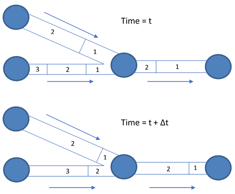
Fig. 12.1 Behavior of segments in the Lagrangian solution method.

The following steps occur within each such time step:

The water quality in each segment is updated to reflect any reaction that may have occurred over the time step.

For each node in topological order (from upstream to downstream):

If the node is a junction or tank, the water from the leading segments of the links with flow into it, if not zero, is blended together to compute a new water quality value. The volume contributed from each segment equals the product of its link’s flow rate and the time step. If this volume exceeds that of the segment, then the segment is destroyed and the next one in line behind it begins to contribute its volume.

If the node is a junction its new quality is computed as its total mass inflow divided by its total inflow volume. If it is a tank, its quality is updated depending on the method used to model mixing in the tank.

The node’s concentration is adjusted by any contributions made by external water quality sources.

A new segment is created in each link with flow out of the node. Its volume equals the product of the link flow and the time step and its quality equals the new quality value computed for the node.

To cut down on the number of segments, new ones are only created if the new node quality differs by a user-specified tolerance from that of the last segment in the outflow link. If the difference in quality is below the tolerance, then the size of the current last segment in the link is simply increased by the volume flowing into the link over the time step and the segment quality is a volume-weighted average of the node and segment quality.

This process is then repeated for the next water-quality time step. At the start of the next hydraulic time step any link experiencing a flow reversal has the order of its segments reversed and if any flow reversal occurs the network’s nodes are re-sorted topologically, from upstream to downstream. Sorting the nodes topologically allows the method to conserve mass in most situations, e.g., even when very short pipes or zero-length pumps and valves are encountered (Davis et al., 2018). Initially each pipe in the network consists of a single segment whose quality equals the initial quality assigned to the upstream node.